3 Simple Programs To Understand CUDA better

It’s no secret that Nvidia unleashed a whole new realm of parallel computing with the CUDA ecosystem. The concept of GPU Computing revolutionized each and every industry vertical reliant on accelerated workloads. It augmented the HPC & AI sphere by leaps and bounds with more friendly means of computing with GPUs. With the growing community support, it has been essential for associated developers/researchers to gain a basic understanding of the same. Hence in this blog, we will help you enter this realm with a few simple programs based on CUDA C/C++.

Pre-Requisites

This article assumes the reader is well versed in C++ (or C). Also, the reader is expected to know basic OS concepts such as threads and processes. A basic idea of what a GPU is, is important. Before we start let’s go through a refresher of the basic CUDA API variables

• threadIdx – A data type that indicates the thread ID of a thread in a kernel
• blockIdx – A data type that indicates the thread block ID of a thread in a kernel
• blockDim – A data type that indicates the thread dimensions of a kernel
• gridDim – A data type that indicates the thread block dimensions of a kernel

(If you’re unaware of these variables read through this first)

Now to begin with, we start off with the simplest example of a CUDA kernel for a warmup element wise operation (vector-vector addition, subtraction etc.)

1.  Element-Wise Vector Operations 

We know in vector addition (BLAS Level 1), we add 2 same length vectors with each other and store the result in a result vector.

Let's say for vectors A, B, C:
A + B = C
Here, A[i] + B[i] = C[i]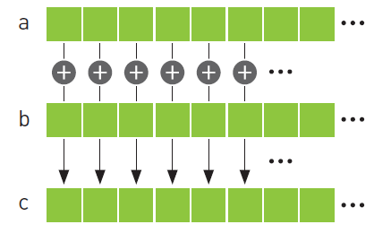

As one can clearly see, each element in the result vector comes from an independent operation that is the sum of the i^th element of the input vectors. Hence, say for an array/vector with 10 elements instead of iterating over the input vectors sequentially from 0…N-1, we can spawn 10 threads and have each thread calculate the i^th element of the resultant array/vector C i.e. in the above operation we replace ‘i’ from an iterator/loop variable to a thread-id variable.

(Shown in the code below) 

__global__ void addKernel(int *c, int *a, int *b)
{
     int i = threadIdx.x;
     c[i] = a[i] + b[i];
}

This kernel is invoked as mentioned below:

addKernel << <1, 10 >> > (c, a, b);

Here, the kernel is launched with 10 threads spawned. Each thread calculates a[thread id] + b[thread id]

Similarly, for subtraction the kernel is mentioned below.

__global__ void subKernel(int* c, int* a, int* b)
{
    int i = threadIdx.x;
    c[i] = a[i] - b[i];
}

Invoking, it in a similar fashion as the add kernel

subKernel << <1, 10 >> > (c, a, b);

Here, each thread calculates: a[thread id] – b[thread id]. Similarly, we can write kernels for multiplication and division.

2. Matrix Multiplication (BLAS Level 3)

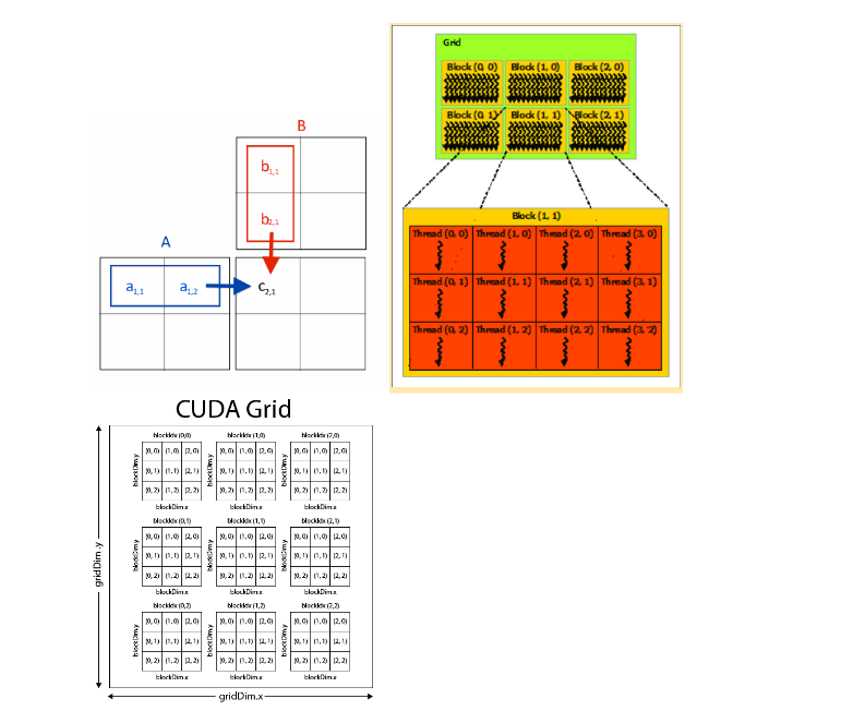
Now, we move on to our second program which is matrix multiplication. As we know, in matrix multiplication the resultant element C[i][j] is calculated by summing the product of adjacent matrices rows and columns.

for (int i=0 ; i<colsizeC ; i++)
    for (int j=0 ; j<rowsizeB ; j++)
        for (int k=0 ; k<colsize ; k++)
            C[i][j] += A[i][k]*B[k][j]

Essentially, the sum of the product of a row of A with a column of B gives the resultant element in C. So here, we spawn a 2D grid of threads where each thread corresponds to an element of the resultant matrix C. Essentially, we parallelise the two outermost for loops. For simplicity of access, we have flattened the 2D matrix to a 1D representation i.e., instead of M[i][j] we have MFlat[i*width+j] (here, width is length of the row)

The kernel is thus formulated as mentioned below.

template<typename T>
__global__
void matrix_multiply(const T* A, const T* B, T* C, int width, int H, int W)
{
    int i = blockIdx.y * blockDim.y + threadIdx.y; //i index threads
    int j = blockIdx.x * blockDim.x + threadIdx.x; //j index threads

    if (i >= H || j >= W) return;

    T localsum = 0;
    for (int k = 0; k < width; k++)
           localsum += A[i * width + k] * B[k * W + j];
    C[i * W + j] = localsum;
}

The above kernel is invoked by generating a kernel with 2D block/grid of threads (unlike our previous example which had 1D grid/block of threads). The following invocation is to multiply two 10×10 matrices together.

matrix_multiply << <1, dim3(10,10,1) >> > (c, a, b);

3. Monte Carlo based Estimation of Pi

Now we move on over from the boring vector operations to something a bit more fun – Estimations with Monte Carlo methods (don’t worry it’s easier than its high-octane name suggests). To proceed with this section, we first need a little catching up on Monte Carlo methods. Monte Carlo methods are essentially probabilistic estimations of deterministic problems i.e., they’re solved by repeated random sampling.

Imagine a 1×1 unit square on a piece of paper. Say, we want to paint it with paintballs. The number of shots required to completely paint over the paper would be inversely proportional to the diameter of the paintballs. Now, imagine the paintballs are point sized (i.e., they have no definable dimensions/radius). As a matter of fact, it would take an infinite number of shots to paint the entire paper.

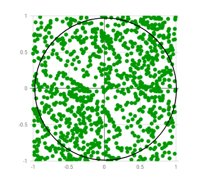
Now, we inscribe a unit circle within the unit square. For these two shapes, if I am to take a point within the square, the probability of the point being inside the circle will be the ratio of the area of the circle and the area of the square.

The area of the circle is (pi*r*r) sq. units and the square has an area of 1 sq. unit. Hence the ratio would be, 0.25*pi. We use these two pieces of information to do a Monte Carlo estimate. We know, 4*P (random dot in circle)/P (dot outside circle) = pi.

Please note, P(x) indicates probability of event x occurring. Now we can estimate those probabilities by simulating a large number of random paintball shots. It will require keeping a track of the balls that hit inside the circle and the total number of balls to estimate the probabilities.

Now the more paintballs we hit, the more accurate we can get our estimate (since infinite would be perfect). So, what we need is a really fast gun to maximize the accuracy of the estimate in a set amount of time.

The algorithm can be better explained by the pseudo-code below.

INTERVAL= 1000
circle_points= 0
square_points= 0
for i in range(INTERVAL**2):
    rand_x= random.uniform(-1, 1)
    rand_y= random.uniform(-1, 1)
    origin_dist= rand_x**2 + rand_y**2
    if origin_dist<= 1:
        circle_points+= 1
    square_points+= 1
    pi = 4* circle_points/square_points

Clearly as each point can be independently calculated, hence parallelisation is possible. So instead of a really fast gun, we use a lot of slower guns together to paint the shapes like a ship’s broadside cannons. 

Now instead of one thread executing the millions of calculations, we have thousands of separate threads doing a couple of hundred/thousand points each. The resultant kernel corresponds to the parallelisation of the previous code.

__global__ void piCount (unsigned long* hits)
{
    curandState_t rng;
    int tid = getthreadid();           //Calculates unique thread ID
    curand_init(clock64(), tid, 0, &rng);
    hits[tid] = 0;
    int counter = 0;
    //Calculating Hits
    for (int i = 0; i < (1<<10); i++)
    {
        float x = curand_uniform(&rng); // Random x position in [0,1]
        float y = curand_uniform(&rng); // Random y position in [0,1]
        counter+= 1 - int(x * x + y * y);
    }
    hits[tid]+=counter;
}

Note: Each thread calculates 1024 hits and stores them in a buffer. At the end all the hits in the buffer are summed up. The kernel can be launched with any configuration depending on how many hits we want to generate.

piCount << <dim3(1, 1, 64), dim3(4, 8, 8) >> > (dOut);

The above configuration simulates (1*1*64) *(4*8*8) *1024 hits or about 16M hits. The following calculation gives the pi estimate from the data generated by the kernel.

int total = 0;
for (int i = 0; i < NBLOCKS; i++)
  total += dOut[i];
unsigned long long tests = (1*1*64) * (4*8*8) * 1024 * (1<<10);
double PI_calced = 4.0 * (double)total / (double)tests;

Note, the summation can also be done parallelly but for simplicity’s sake it was done with a simple for loop.

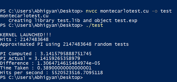
Benchmark

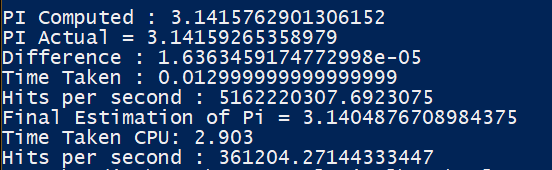
Understanding CUDA is fine, but what’s the point if we don’t get to see it in action? How much benefit are we getting by going through all the hassle of parallelisation? Therefore, let’s launch the small guns and run one of the examples discussed above. The screenshots below, elucidate the execution time (in seconds) of both serial and parallel versions of Monte Carlo estimation.

Takeaways

Hope, this blog provided you with a basic knowledge of leveraging CUDA C/C++ for HPC. To summarise, here is what we learnt.

• Benefits of parallelism.
• CUDA jargons.
• Parallel approach to vector addition/substraction & multiplication
• Accelerated Monte-Carlo estimation